MsRaster

MsRaster is an application for 2-dimensional raster visualization and flagging of visibility and spectrum data. This data must be in a Zarr file using the XRADIO MSv4 schema. An input path for the MeasurementSet v2 table format will be automatically converted to MeasurementSet v4 if the necessary packages for the conversion are installed.

Implementation

Application Modes

MsRaster creates raster plots for the user to view interactively or save to disk. The application can be used in three ways from Python:

create raster plots to export to file
create interactive Bokeh raster plots to show in a browser window
use a GUI dashboard in a browser window to select plot parameters and create interactive Bokeh raster plots

Data Exploration

XRADIO allows the user to explore MeasurementSet data with a summary of its metadata, and to make plots of antenna positions and phase center locations of all fields. These features can be accessed in MsRaster, as well as the ability to list MSv4 data groups and dimension values to aid in selection.

Raster Plots

MsRaster gives the user flexibility to select data, style the plots, set plot axes and the complex component, aggregate along one or more data dimensions, iterate along a data dimension, and layout multiple plots in a grid. All plot parameters available from the MsRaster methods are available in the interactive GUI. When a single plot is shown, the metadata for the cursor position will be displayed below the plot. Points and boxes may be drawn, and the metadata for each point in these regions will be displayed in tabs. These regions may also be selected for flagging.

Using MsRaster to Create Plots

In this simple example with no GUI, we import MsRaster, construct an MsRaster object, create a raster plot with default parameters, and show the interactive Bokeh plot in a browser tab:

>>> from vidavis import MsRaster
>>> msr = MsRaster(ms=myms)
>>> msr.plot()
>>> msr.show()

Construct MsRaster Object

>>> msr = MsRaster(ms=None, log_level='info', log_to_file=True, show_gui=False)

ms (str): path to MSv4 (usually .zarr extension) or MSv2 (usually .ms extension) file. Required when show_gui=False.
log_level (str): logging threshold. Options include ‘debug’, ‘info’, ‘warning’, ‘error’, ‘critical’. Default ‘info’.
log_to_file (bool): whether to write log messages to a log file. Default True.
show_gui (bool): whether to launch the interactive GUI in a browser tab. Default False.

MsRaster can be constructed with the ms path to a MSv4 or MSv2 file. If a MSv2 path is supplied and the correct dependencies have been installed separately (see Install for MSv2 Conversion), the MSv2 will automatically be converted to the MSv4 Zarr format in the same directory as the MSv2, with the extension .ps.zarr. For more information on the MSv4 data format, see the XRADIO Measurement Set Tutorial.

Warning

MSv2 files will be converted to Zarr using the XRADIO default partitioning: data description (spectral window and polarization setup) and observation mode. For other partitioning, you may convert the MSv2 to Zarr prior to using MsRaster.

The log_level can be set to the desired level, with log messages output to the Python console. When the log_to_file option is True (default), log messages will also be written to the file msraster-<timestamp>.log in the current directory.

At construction, set whether plot parameters will be set in the Python console or a script (showgui is False) or in the interactive GUI (showgui is True). When the GUI is shown, using MsRaster functions will not update the GUI input parameters or the plot. The ms parameter is required when showgui is False, but optional when this path can be set in the GUI.

Explore MS Data

MsRaster may be used to explore the MeasurementSet for plotting. The .zarr file is opened as an XRADIO ProcessingSetXdt, which is an Xarray DataTree (Xdt) composed of MSv4 DataTrees (see Measurement Set Tutorial for more information). The XRADIO custom functions for data exploration in ProcessingSetXdt are available in MsRaster.

Some functions require that the MSv4 data groups name is specified. Data groups are a set of related visibility/spectrum data, uvw, flags, and weights. To see the available data groups in the ProcessingSetXdt:

>>> msr.data_groups(show=False)

show (bool): whether to show the data groups in a readable format, or return the data groups dictionary. Default False (return the dictionary).

The following examples are for a dataset with base, corrected, and model data groups:

>>> groups = msr.data_groups()
>>> groups
{'base': {'correlated_data': 'VISIBILITY', 'date': '2025-08-19T18:06:03.322237+00:00', 'description': "Data group derived from the data column 'VISIBILITY' of an MSv2 converted to MSv4", 'field_and_source': 'field_and_source_base_xds', 'flag': 'FLAG', 'uvw': 'UVW', 'weight': 'WEIGHT'}, 'corrected': {'correlated_data': 'VISIBILITY_CORRECTED', 'date': '2025-08-19T18:06:03.322249+00:00', 'description': "Data group derived from the data column 'VISIBILITY_CORRECTED' of an MSv2 converted to MSv4", 'field_and_source': 'field_and_source_corrected_xds', 'flag': 'FLAG', 'uvw': 'UVW', 'weight': 'WEIGHT'}, 'model': {'correlated_data': 'VISIBILITY_MODEL', 'date': '2025-08-19T18:06:03.322251+00:00', 'description': "Data group derived from the data column 'VISIBILITY_MODEL' of an MSv2 converted to MSv4", 'field_and_source': 'field_and_source_model_xds', 'flag': 'FLAG', 'uvw': 'UVW', 'weight': 'WEIGHT'}}
>>> msr.data_groups(show=True)
base :
    correlated_data = VISIBILITY
    date = 2025-08-19T18:06:03.322237+00:00
    description = Data group derived from the data column 'VISIBILITY' of an MSv2 converted to MSv4
    field_and_source = field_and_source_base_xds
    flag = FLAG
    uvw = UVW
    weight = WEIGHT
corrected :
    correlated_data = VISIBILITY_CORRECTED
    date = 2025-08-19T18:06:03.322249+00:00
    description = Data group derived from the data column 'VISIBILITY_CORRECTED' of an MSv2 converted to MSv4
    field_and_source = field_and_source_corrected_xds
    flag = FLAG
    uvw = UVW
    weight = WEIGHT
model :
    correlated_data = VISIBILITY_MODEL
    date = 2025-08-19T18:06:03.322251+00:00
    description = Data group derived from the data column 'VISIBILITY_MODEL' of an MSv2 converted to MSv4
    field_and_source = field_and_source_model_xds
    flag = FLAG
    uvw = UVW
    weight = WEIGHT

The ProcessingSetXdt metadata for one of the MSv4 data groups name can be displayed in a tabular format. These column names and values can be used to select the ProcessingSetXdt (see select_ps() in Select Raster Data):

>>> msr.summary(data_group='base', columns=None)

data_group (str): name of data group for summary. Default ‘base’.
columns (str, list, None): which summary columns to display. Default None shows all columns. Column names may be selected with a string or list. Setting columns to ‘by_ms’ displays the summary in a readable format for each MeasurementSetXdt in the ProcessingSetXdt.

By default, the entire summary for the base data group is shown:

>>> msr.summary()
                    name  \
sis14_twhya_selfcal_0
sis14_twhya_selfcal_1
sis14_twhya_selfcal_2
sis14_twhya_selfcal_3

                                                                         scan_intents  \
[CALIBRATE_BANDPASS#ON_SOURCE, CALIBRATE_PHASE#ON_SOURCE, CALIBRATE_WVR#ON_SOURCE]
   [CALIBRATE_AMPLI#ON_SOURCE, CALIBRATE_PHASE#ON_SOURCE, CALIBRATE_WVR#ON_SOURCE]
                              [CALIBRATE_PHASE#ON_SOURCE, CALIBRATE_WVR#ON_SOURCE]
                                                        [OBSERVE_TARGET#ON_SOURCE]

                shape      execution_block_UID polarization  \
 (40, 210, 384, 2)  uid://A002/X554543/X207     [XX, YY]
 (20, 190, 384, 2)  uid://A002/X554543/X207     [XX, YY]
 (80, 210, 384, 2)  uid://A002/X554543/X207     [XX, YY]
(270, 210, 384, 2)  uid://A002/X554543/X207     [XX, YY]

                          scan_name                          spw_name  \
                         [33, 4]  ALMA_RB_07#BB_2#SW-01#FULL_RES_0
                             [7]  ALMA_RB_07#BB_2#SW-01#FULL_RES_0
[10, 14, 18, 22, 26, 30, 34, 38]  ALMA_RB_07#BB_2#SW-01#FULL_RES_0
        [12, 16, 20, 24, 28, 36]  ALMA_RB_07#BB_2#SW-01#FULL_RES_0

     spw_intents              field_name               source_name line_name  \
[UNSPECIFIED]  [3c279_6, J0522-364_0]  [J0522-364_0, Unknown_5]        []
[UNSPECIFIED]               [Ceres_2]             [J1037-295_2]        []
[UNSPECIFIED]           [J1037-295_3]                [TW Hya_3]        []
[UNSPECIFIED]              [TW Hya_5]                 [3c279_4]        []

                         field_coords session_reference_UID  \
                Multi-Phase-Center                   ---
  [fk5, 6h10m15.95s, 23d22m06.91s]                   ---
[fk5, 10h37m16.08s, -29d34m02.81s]                   ---
[fk5, 11h01m51.80s, -34d42m17.37s]                   ---

     scheduling_block_UID             project_UID  start_frequency  \
uid://A002/X327408/X73  uid://A002/X327408/X6f     3.725331e+11
uid://A002/X327408/X73  uid://A002/X327408/X6f     3.725331e+11
uid://A002/X327408/X73  uid://A002/X327408/X6f     3.725331e+11
uid://A002/X327408/X73  uid://A002/X327408/X6f     3.725331e+11

   end_frequency
 3.727669e+11
 3.727669e+11
 3.727669e+11
 3.727669e+11

If a subset of columns is of interest, set columns to one or more column names:

>>> msr.summary(data_group='base', columns='intents')
>>> msr.summary(data_group='base', columns=['spw_name', 'shape'])
>>> msr.summary(data_group='base', columns=['spw_name', 'start_frequency', 'end_frequency'])

To view the summary information grouped by MSv4, set columns to ‘by_ms’ (only the first MS is shown here):

>>> msr.summary(data_group='base', columns='by_ms')
name: sis14_twhya_selfcal_0
scan_intents: ['CALIBRATE_BANDPASS#ON_SOURCE', 'CALIBRATE_PHASE#ON_SOURCE', 'CALIBRATE_WVR#ON_SOURCE']
shape: 40 times, 210 baselines, 384 channels, 2 polarizations
execution_block_UID: uid://A002/X554543/X207
polarization: ['XX' 'YY']
scan_name: ['33', '4']
spw_name: ALMA_RB_07#BB_2#SW-01#FULL_RES_0
spw_intents: ['UNSPECIFIED']
field_name: ['3c279_6', 'J0522-364_0']
source_name: ['J0522-364_0', 'Unknown_5']
line_name: []
field_coords: (M) u l
session_reference_UID: ---
scheduling_block_UID: uid://A002/X327408/X73
project_UID: uid://A002/X327408/X6f
frequency range: 3.725331e+11 - 3.727669e+11

The values in each data dimension may be listed:

>>> msr.get_dimension_values(dimension)

dimension (str): which dimension to list. Options include ‘time’, ‘baseline’, ‘frequency’, and ‘polarization’. Baseline antennas may be listed separately with ‘antenna1’ and ‘antenna2’.

The list of dimension values can be used to select data in the MeasurementSetXdts (see select_ms() in Select Raster Data):

>>> msr.get_dimension_values('polarization')
['XX', 'YY']
>>> msr.select_ms(polarization='XX')

The ‘time’ dimension is returned as datetime strings in the format dd-Mon-YYYY HH:MM:SS. Use this format to select time in select_ms().

The ‘baseline’ dimension is returned as strings in the format antenna1 & antenna2. Use this format to selection baseline in select_ms().

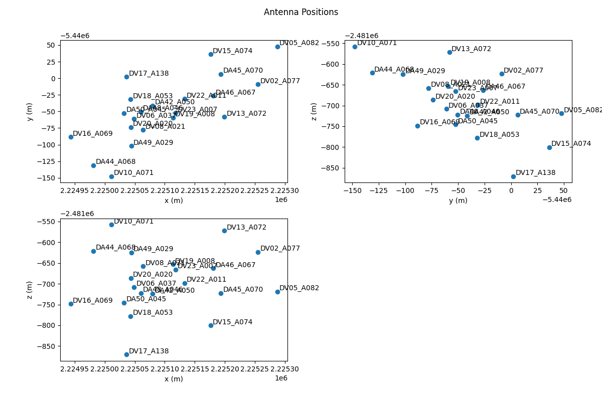
MsRaster includes the XRADIO ProcessingSetXdt function to plot antenna positions, optionally labeled by name:

>>> msr.plot_antennas(label_antennas=False)

label_antennas (bool): whether to label each antenna in the antenna position plot. Default False.

Without antenna labels, the name can be shown by hovering over an antenna position. Example plot with antenna labels:

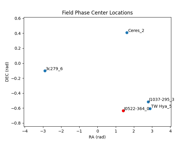
MsRaster also includes the XRADIO ProcessingSetXdt function plot_phase_centers(), which plots the phase center locations of all fields in a data group:

>>> msr.plot_phase_centers(data_group='base', label_fields=False)

data_group (str): name of data group with field_and_source_xds to plot. Default ‘base’.
label_fields (bool): Whether to label each field in the plot.

When label_fields is False, the central field is highlighted in red based on the closest phase center calculation, and the legend shows the central field name. Otherwise, all fields are named and the central field is red. Sample plot with label_fields set to True:

Style Raster Plots

Plot style settings may be set and will be used for all plots. Currently, the style includes colormaps and whether to show colorbars for unflagged and flagged data.

>>> msr.set_style_params(unflagged_cmap='Viridis', flagged_cmap='Reds',
show_colorbar=True, show_flagged_colorbar=True)

unflagged_cmap (str): colormap for unflagged data. Default ‘Viridis’.
flagged_cmap (str): colormap for flagged data. Default ‘Reds’.
show_colorbar (bool): whether to show the colorbar for unflagged data. Default True.
show_flagged_colorbar (bool): whether to show the colorbar for flagged data. Default True.

The show the list of available colormaps:

>>> msr.colormaps()
['Blues', 'Cividis', 'Greens', 'Greys', 'Inferno', 'Magma', 'Oranges',
'Plasma', 'Purples', 'Reds', 'Turbo', 'Viridis']

In the future, additional style settings may be available and these settings may be able to be stored in a configuration file rather than set each time.

Select Raster Data

MsRaster has two ways to select data: select_ps() to select a subset of MeasurementSetXdts in the ProcessingSetXdt, and select_ms() to select data in the MeasurementSetXdts. Use either method to select one of the available data groups using keyword data_group_name (see data_groups).

Select ProcessingSetXdt

Processing set selection is based on the summary and filters the MeasurementSetXdts in the ProcessingSetXdt:

select_ps(string_exact_match=True, query=None, **kwargs)

string_exact_match (bool): whether to require exact matches for string values (default True) or allow partial matches (False).
query (str): a Pandas query string to apply additional filtering.
kwargs (dict): keyword arguments representing summary column names and values.

Since the summary is a Pandas dataframe, a Pandas query string may be used to filter the MeasurementSetXdts included in a ProcessingSetXdt. Keyword arguments (kwargs) use summary column names and data_group_name to select the ProcessingSetXdt:

>>> msr.select_ps(query='start_frequency > 100e9 AND end_frequency < 200e9')
>>> msr.select_ps(data_group_name='corrected', field_name='TW Hya_5', scan_name='16', polarization='XX')

The keyword arguments may be passed as a Python dictionary:

>>> ps_selection = {'field_name': 'TW Hya_5', 'scan_name': '16', 'polarization': 'XX'}
>>> msr.select_ps(**ps_selection)

The keyword values may be a single value as shown above, or a list of values:

>>> msr.select_ps(scan_name=['16', '18', '20'])

With ProcessingSetXdt selection, the option for an exact string match (default) or a partial string match for string values is available using the string_exact_match parameter:

>>> msr.select_ps(string_exact_match=False, query=None, intents='CALIBRATE_BANDPASS')
>>> msr.select_ps(string_exact_match=False, query=None, field_name='Venus')

Note the ProcessingSetXdt selection is not applied to the data in the MeasurementSetXdts, unless exact_string_match is True and the column name is ‘polarization’, ‘scan_name’, or ‘field_name’.

For additional explanation and examples, see also query() in the ProcessingSetXdt API.

Select MeasurementSetXdt

MeasurementSetXdt selection is based on xarray.Dataset.sel using data groups and dimensions:

>>> msr.select_ms(indexers=None, method=None, tolerance=None, drop=False, **indexers_kwargs)

indexers (dict): a dict with keys matching dimensions and values given by scalars, slices or arrays.
method (str): method to use for inexact matches: None (only exact matches), ‘pad’/’ffill’ (propagate last valid index value forward), ‘backfill’/’bfill’ (propagate next valid index value backward), ‘nearest’ (use nearest valid index value). Default None.
tolerance (float): maximum distance between original and new values for inexact matches.
drop (bool): whether to drop coordinate variables in indexers instead of making them scalar. Default False.
indexers_kwargs: the keyword arguments form of indexers. indexers or indexers_kwargs must be provided.

Indexer keywords include data_group_name and dimensions time, baseline (for visibilities), antenna_name (for spectrum), frequency, and polarization. Use get_dimension_values for a list of valid dimension values to select. A set of baselines may also be selected by antenna with antenna1 and antenna2:

>>> msr.select_ms(antenna1='DA44_A068')

Numeric value selection supports inexact matches using parameters method and tolerance. Here, the nearest frequency value within 100 MHz of 372.6 GHz is selected:

>>> msr.select_ms(frequency=3.726e+11, method='nearest', tolerance=1e+8)

Values may be a single value, a list, or a slice. Time selection must be in string format ‘dd-Mon-YYYY HH:MM:SS’ as shown in get_dimension_values('time'):

>>> msr.select_ms(polarization=['XX', 'YY']
>>> msr.select_ms(time=slice('19-Nov-2012 09:00:00', '19-Nov-2012 09:12:00'))

For additional explanation and examples, see sel() in the MeasurementSetXdt API.

Warning

All selections using select_ps() and select_ms() are cumulative, with each selection acting on the previously-selected ProcessingSetXdt and MeasurementSetXdts.

To clear previous selections and return to the original ProcessingSetXdt:

>>> msr.clear_selection()

Note

Automatic selection: Since MsRaster creates a 2D plot from 4D data, some selections must be done automatically if not selected by the user. These selections include:

spw name: for consistent data shapes, the first spectral window (by time) is selected.

data group: default ‘base’.

data dimensions: the dimensions which have not been chosen for x_axis, y_axis, aggregation agg_axis or iteration iter_axis are automatically selected. After user selections are applied, the set of dimension values are sorted, and the first is used. Time and frequency are numeric values. For baseline, names are formed as ‘ant1_name & ant2_name’ strings and sorted, then the first pair in the list is selected. For polarization, the names are converted to casacore Stokes enum values, sorted, and the first in the list is selected and converted back to a name for value selection.

Create Raster Plot

Use plot() to create each raster plot, which can then be shown (see Show Raster Plot) or saved (see Save Raster Plot):

>>> msr.plot(x_axis='baseline', y_axis='time', vis_axis='amp', aggregator=None,
agg_axis=None, iter_axis=None, iter_range=None, subplots=None, color_mode=None,
color_range=None, title=None, clear_plots=True)

x_axis, y_axis (str): select the axes to plot from the data dimensions ‘time’, ‘baseline’ (for visibility data), ‘antenna_name’ (for spectrum data), ‘frequency’, and ‘polarization’. Default x_axis is ‘baseline’, equivalent to ‘antenna_name’ for spectrum data. Default y_axis is ‘time’.
vis_axis (str): the complex component of the visibility data has options ‘amp’, ‘phase’, ‘real’, and ‘imag’. For spectrum data, only ‘amp’ and ‘real’ are valid. Default is ‘amp’, equivalent to ‘real’ for spectrum data.
aggregator (None, str): the reduction function to apply along the agg_axis dimension(s) of all correlated data in the data group. Aggregator options include ‘max’, ‘mean’, ‘min’, ‘std’, ‘sum’, and ‘var’. The reduction is applied after the vis_axis component is calculated. Flags and weights are not used in the aggregation but are aggregated. Default None.
agg_axis (None, str, list): which dimension(s) to apply the aggregator across. Cannot include x_axis or y_axis. Ignored if aggregator is None. The entire dimension(s) are aggregated. If agg_axis is a single dimension, the remaining dimension is selected automatically as described above. If agg_axis is None, all remaining dimensions are aggregated. Default None.
iter_axis (None, str): dimension along which to iterate to create multiple plots. Cannot be x_axis or y_axis. Select the iteration index range with iter_range. Default None.
iter_range (None, tuple): (start, end) inclusive index values for creating iteration plots. Use (0, -1) for all iterations. Warning: you may trigger a MemoryError with many iterations. Iterated plots can be shown or saved in a grid (see subplots) or saved individually (see Save Raster Plot). Default None is equivalent to (0, 0), first iteration only.
subplots (None, tuple): set a plot layout of (rows, columns). Use when multiple plots are created with iter_axis and iter_range, or with clear_plots set to False. If the layout size is less than the number of plots, subplots will limit the plots shown in the layout. If the number of plots is less than the subplots size, the plots will appear in the layout according to the number of columns but fewer or incomplete rows. When multiple plots are created when clear_plots is False, the last subplots setting will be used for the layout. Default None is equivalent to (1, 1), a single plot.
color_mode (None, str): whether to limit the colorbar range for amplitudes. Options include None (use data limits), ‘auto’ (calculate limits for amplitude), and ‘manual’ (use color_range). ‘auto’ is equivalent to None if vis_axis is not ‘amp’. ‘manual’ is equivalent to None if color_range is None. Automatic limits for amplitudes are calculated from statistics for the unflagged data in the spectral window, which uses GraphVIPER MapReduce for fast computation. The range is clipped to 3-sigma limits to brighten weaker data values. Default None (use data limits).
color_range (None, tuple): (min, max) of colorbar to use if color_mode is ‘manual’, else ignored. Default None (use data limits).
title (None, str): plot title. Options include None, ‘ms’ (generate a title from the ms name, appended with iter_axis value if any), or a custom title string. Default None (no plot title).
clear_plots (bool): whether to clear the list of any previous plot(s). Set to False to create multiple plots and show them in a layout with subplots. This option is not currently available in the interactive GUI. Default True (remove previous plots).

Examples:

Aggregation: time vs. baseline averaged over frequency, with the first polarization selected automatically:
```
>>> msr.plot(x_axis='baseline', y_axis='time', aggregator='mean', agg_axis='frequency')
```

Aggregation: time vs. baseline averaged over frequency, with polarization selection:

>>> msr.plot(x_axis='baseline', y_axis='time', selection={'polarization': 'YY'},
aggregator='mean', agg_axis='frequency')

Aggregation: time vs. baseline averaged over frequency and polarization (equivalent to agg_axis=['frequency', 'polarization']):
```
>>> msr.plot(x_axis='baseline', y_axis='time', aggregator='mean')
```
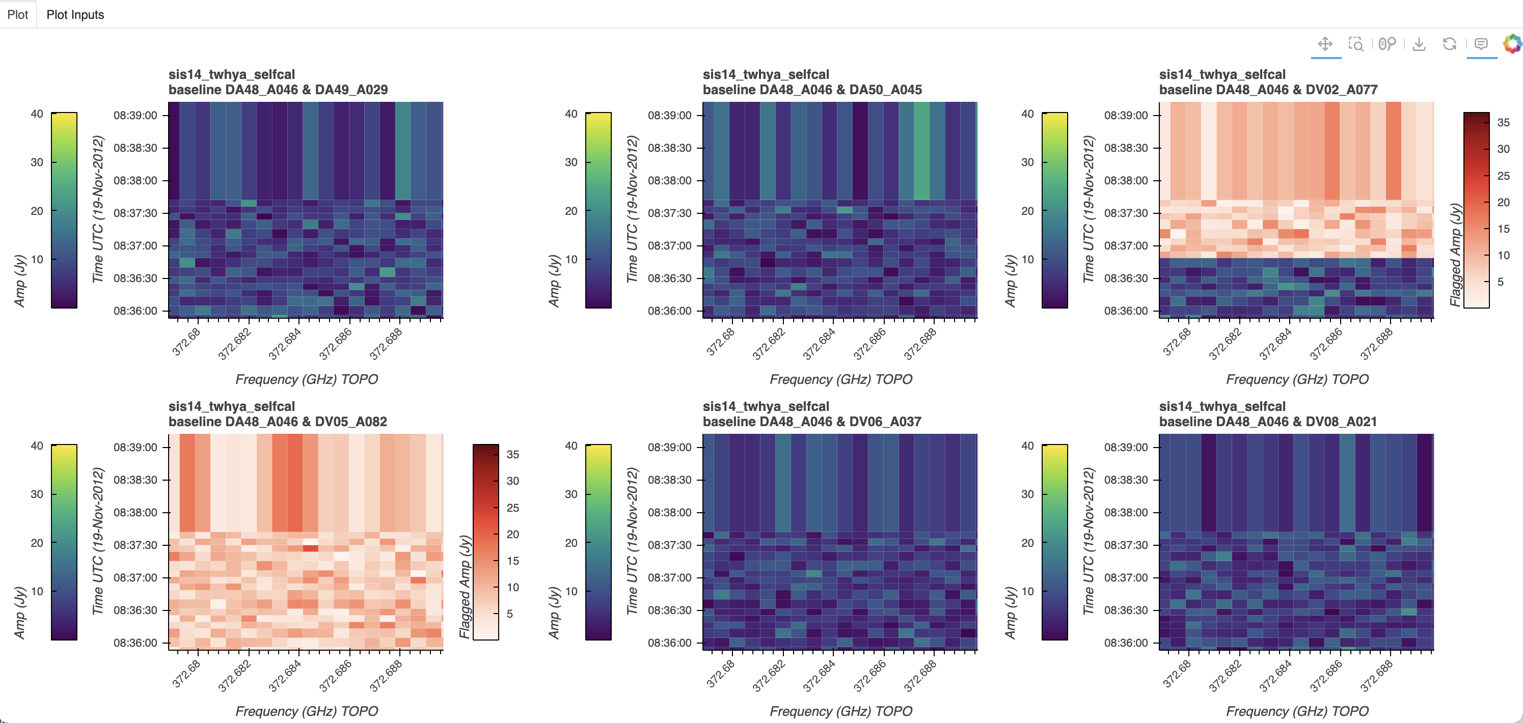
Iteration layout: time vs. baseline for the first six frequencies in 2 rows, with the first polarization selected automatically:
```
>>> msr.plot(iter_axis='frequency', iter_range=(0, 5), subplots=(2, 3))
```
Multiple plots layout: time vs. baseline for ‘amp’ and ‘phase’ in one row, with the first frequency and polarization selected automatically:
```
>>> msr.plot(vis_axis='amp')
>>> msr.plot(vis_axis='phase', subplots=(1, 2), clear_plots=False)
```

Aggregation and iteration layout: time vs. frequency for the max across baselines, iterated over all polarizations, in a 2x2 layout with a clipped colorbar range:

>>> msr.plot(x_axis='frequency', y_axis='time', vis_axis='amp', aggregator='max',
agg_axis='baseline', iter_axis='polarization', iter_range=(0, -1), subplots=(2, 2),
color_mode='auto')

Show Raster Plot

After an interactive Bokeh plot is created (see Create Raster Plot), it may be shown in a browser tab with show(), which has no parameters:

>>> msr.show()

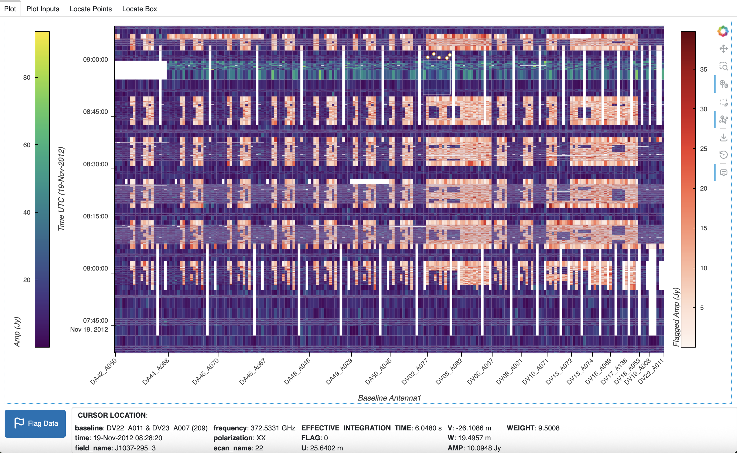
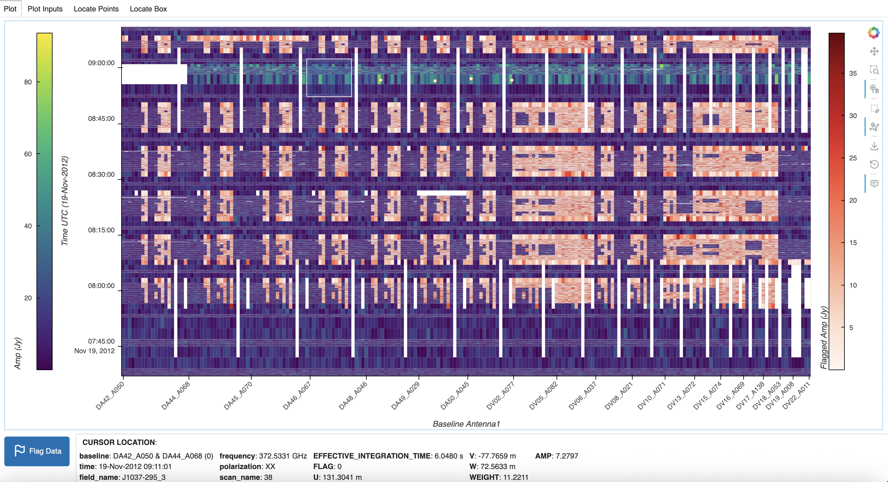
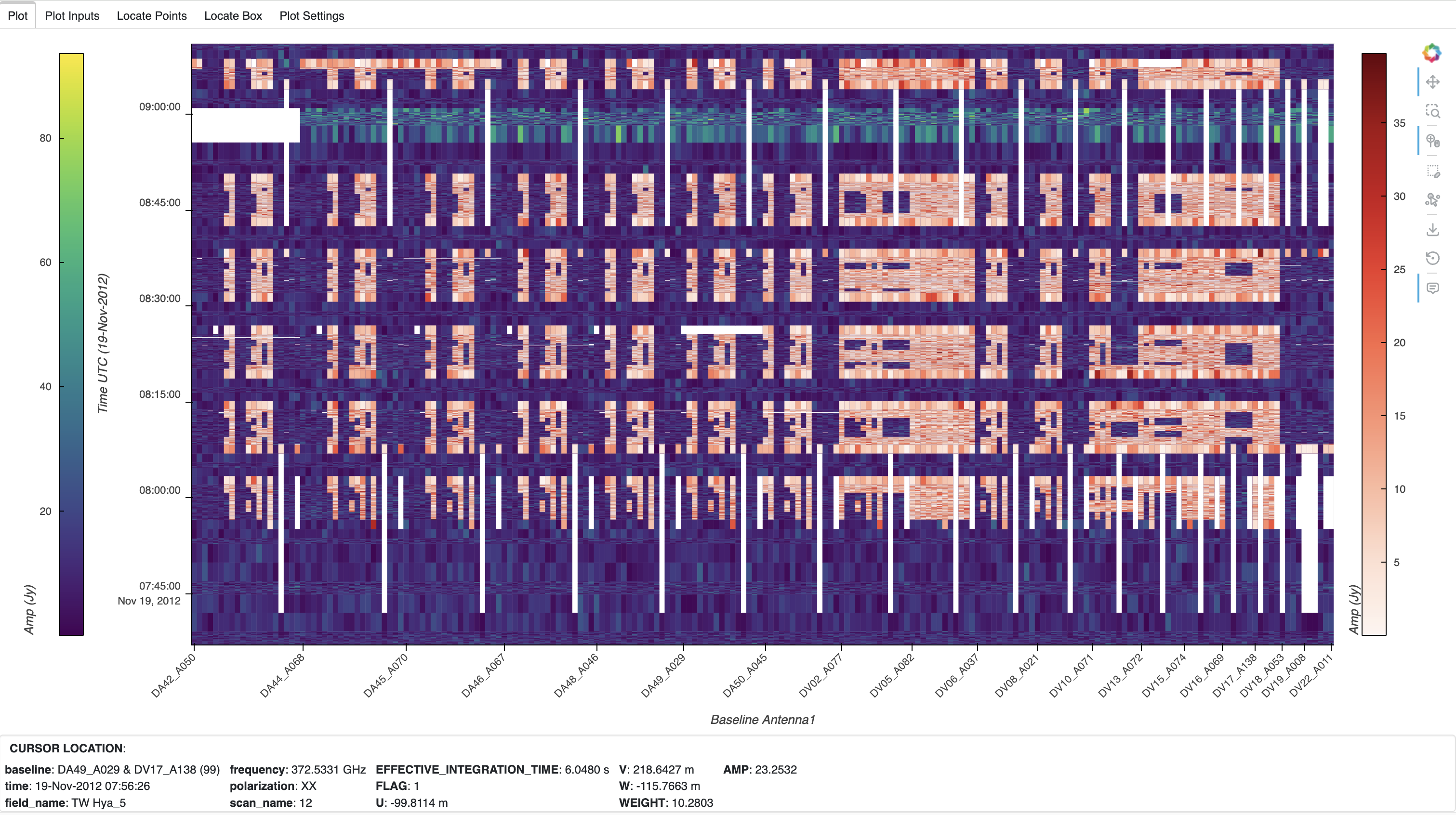
To show the plot, Holoviews renders the plot and saves it to an HTML file in a temporary directory, then automatically opens the file in the browser. The white areas in this plot contain no data, and the hover tool shows the plot data at the cursor position (x, y, and vis axis values):

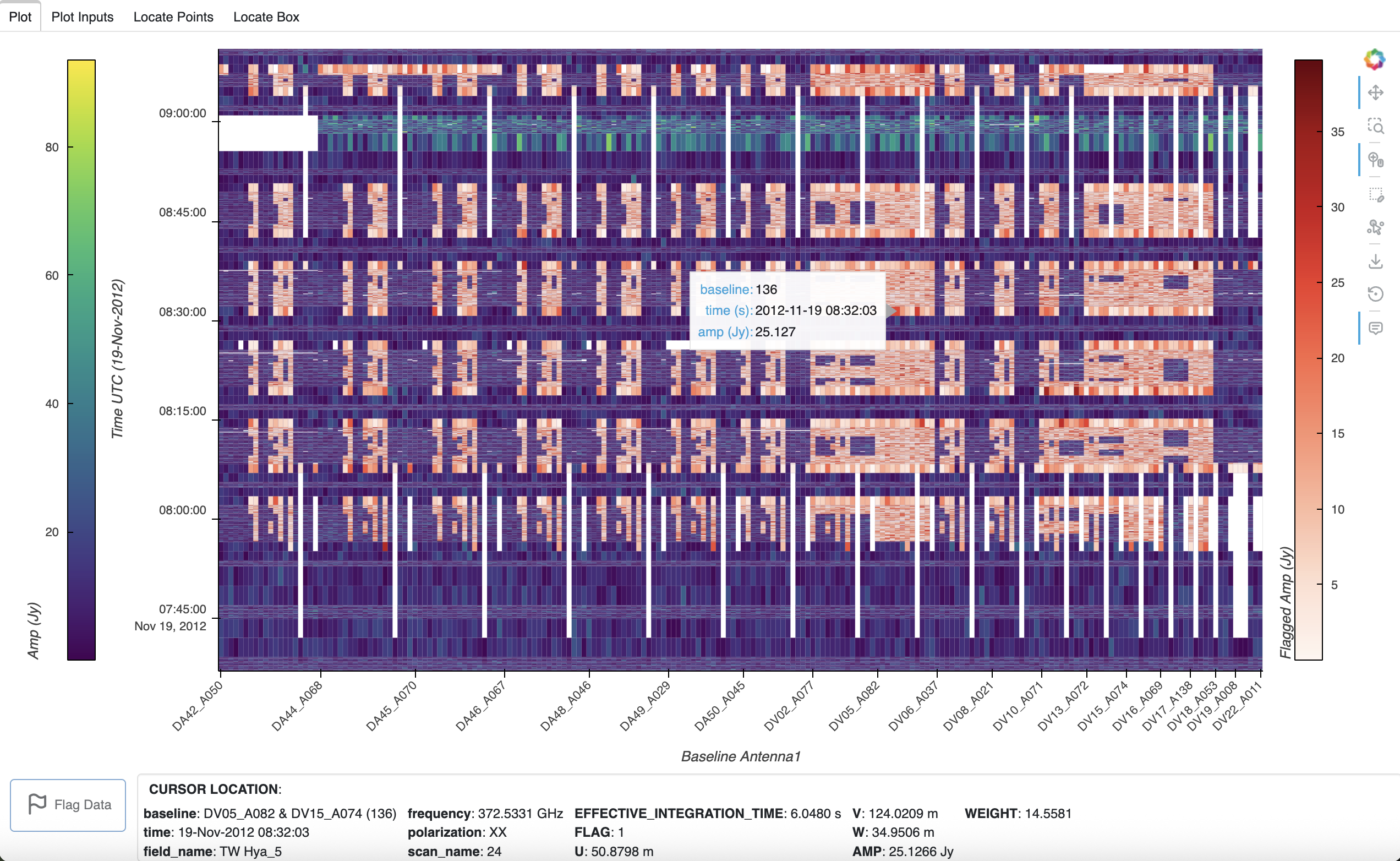
To the right of the plot, the toolbar contains the Bokeh icons for plot tools. At the top of the toolbar, the Bokeh icon is a link to the Bokeh website, and below it in order are the pan, box zoom, wheel zoom, box edit, point draw, save, reset, and hover tool icons. By default, the pan, wheel zoom, and hover tools are activated for the plot, indicated by the line to the left of the icons. Bokeh plot tools can be enabled or disabled by clicking on the tool icon.

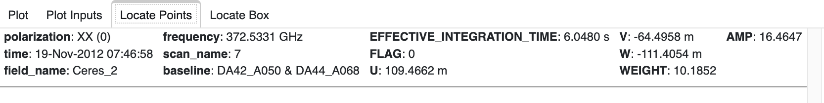
In addition to the hover information, when the cursor moves over the plot, a Cursor Location box appears under the plot to show the coordinates and data variables associated with the cursor position.

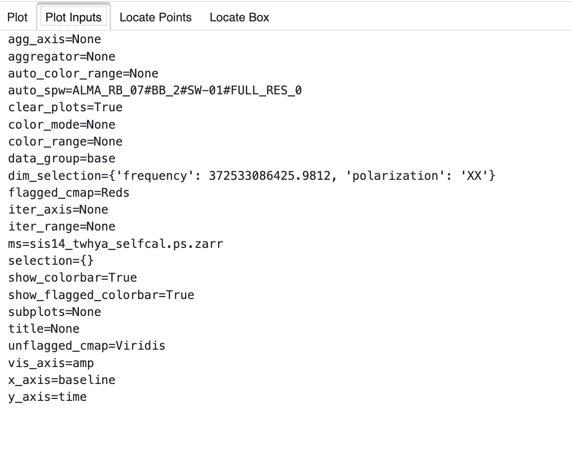
The plot is shown with four tabs at the upper left. The first tab (Plot), which is active by default, contains the plot and the cursor location box. The second tab (Plot Inputs) shows the parameters used to make the raster plot (including automatic selections), sorted alphabetically:

The remaining tabs are for showing the location of points selected in the plot by point or box. See Locate Plot Data for a detailed description.

Note

The Locate features are disabled in a plot when a new plot is created with plot(), since the plot data needed for the metadata is no longer available. The cursor box and locate tabs are removed, but the hover tool is still active. The new plot is shown in a new tab with Locate features.

If multiple plots were created (with iter_axis, or clear_plots set to False) in a subplots layout, the plots are connected so that the Bokeh plot tools such as pan and zoom act on all plots in the layout. The following layout of a dataset iterated by baseline demonstrates the same zoom level in all plots, with the shared toolbar at the upper right:

Note

The Locate features are not available when multiple plots are shown in a layout, but the Hover tool is active.

Locate Plot Data

Location information can be shown for the current cursor position, points drawn using the Point Draw tool, and points contained in a box drawn with the Box Edit tool. Only one selection tool can be active; selection tools include Pan, Box Zoom, Box Edit, and Point Draw. Activating a new selection tool will deactivate the previous selection tool.

Cursor:

When the cursor is positioned over the plot, the hover values are shown in the plot, and additional Cursor Location information appears under the plot.

Draw Points:

Any number of points may be drawn, moved, or deleted by activating the Point Draw tool.

Add point: Tap anywhere on the plot.
Move point: Tap and drag an existing point. The point will be dropped once you let go of the mouse button.
Delete point: Tap a point to select it then press BACKSPACE key while the mouse is within the plot area.

You may need to zoom in to select a point rather than drawing a new point. Using the Bokeh Reset tool on the toolbar to reset the pan or zoom level will not delete the points.

Draw Box:

Boxes may be drawn, moved, or deleted by activating the Box Edit tool.

Add box: Hold shift then click and drag anywhere on the plot or press once to start drawing, move the mouse and press again to finish drawing.
Move box: Click and drag an existing box, the box will be dropped once you let go of the mouse button.
Delete box: Tap a box to select it then press BACKSPACE key while the mouse is within the plot area.

To Move or Delete multiple boxes at once:

Move selection: Select box(es) with SHIFT+tap then drag anywhere on the plot. Selecting and then dragging on a specific box will move both.
Delete selection: Select box(es) with SHIFT+tap then press BACKSPACE while the mouse is within the plot area.

Using the Bokeh Reset tool on the toolbar to reset the pan or zoom level will not delete the boxes.

In the following plot, a box and several points (small white circles above the box) are selected in the plot, and the Point Draw tool is activated:

Locate Points:

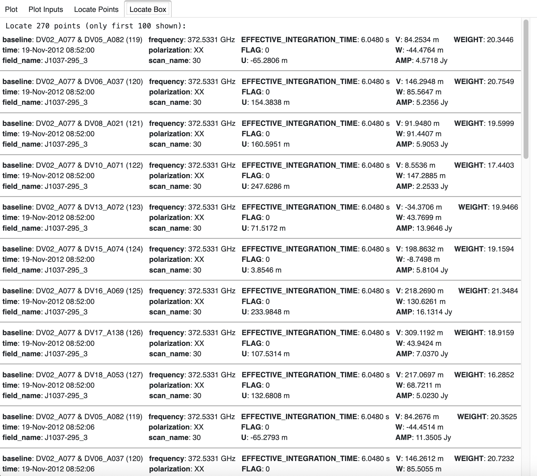
The location information for points is automatically displayed in the Locate tabs and in the log file. Points drawn individually with Point Draw will appear in the third tab (Locate Points), and points in a box drawn with Box Edit will appear in the fourth tab (Locate Box).

The location information includes the coordinate and data variable information associated with each point. For example, in the Locate Box tab, the number of points in the box is shown, then the points are listed with a divider between them. Only the first 100 points in the selected box are located, starting with the first row of the box.

Warning

The Locate Box tab will remain blank or contain the previous box points until the location information for the new points is obtained and formatted, then the tab is updated.

Although multiple boxes may be selected by pressing the SHIFT key, the list of points for each box in the Locate Box tab will be cleared with each new box selection rather than appended. However, the locations for the points in a box can be accessed in the log file, in the order the boxes are created.

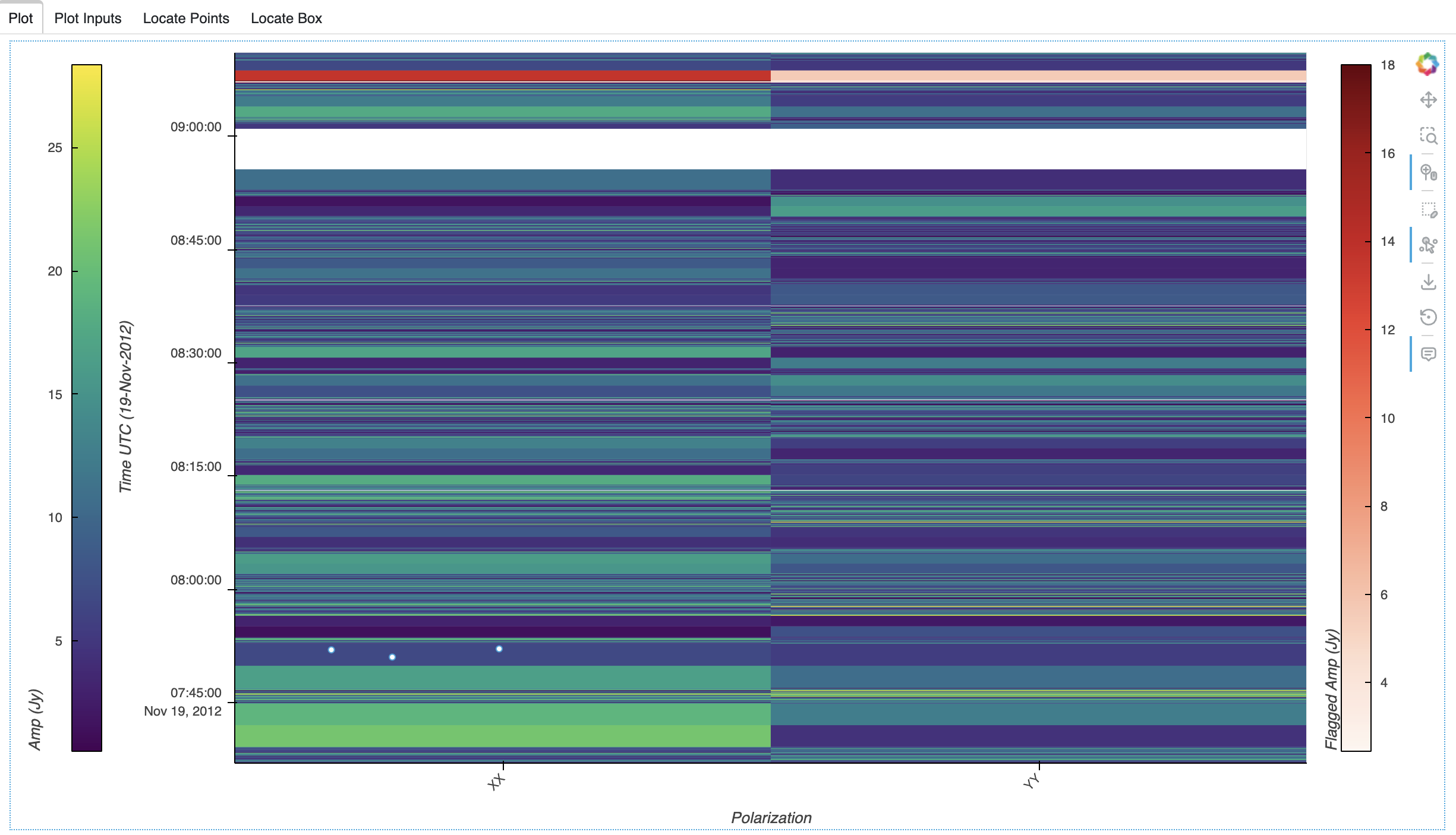
It is possible to draw multiple points for the same data location. All points will exist on the plot, but only one point is located. For example, the points in this plot have the same polarization and timestamp, so one location is shown in the Locate Points tab:

../_images/msraster_duplicate_points.png

../_images/msraster_duplicate_points_locate.png

Flag Plot Data

When points and/or boxes are drawn on the plot and located, as described in Locate Plot Data, these point and box regions may be selected for flagging. Once the data in the regions have been located in the corresponding Locate tabs, the Flag Data button at the lower left will be enabled (signified by a solid button rather than an outline):

When the Flag Data button is clicked, a dialog is opened on the plot for the flagging parameters. This dialog box may be dragged anywhere in the browser tab, and using the control buttons in the upper right, may be (in left to right order) collapsed, minimized, maximized, or closed.

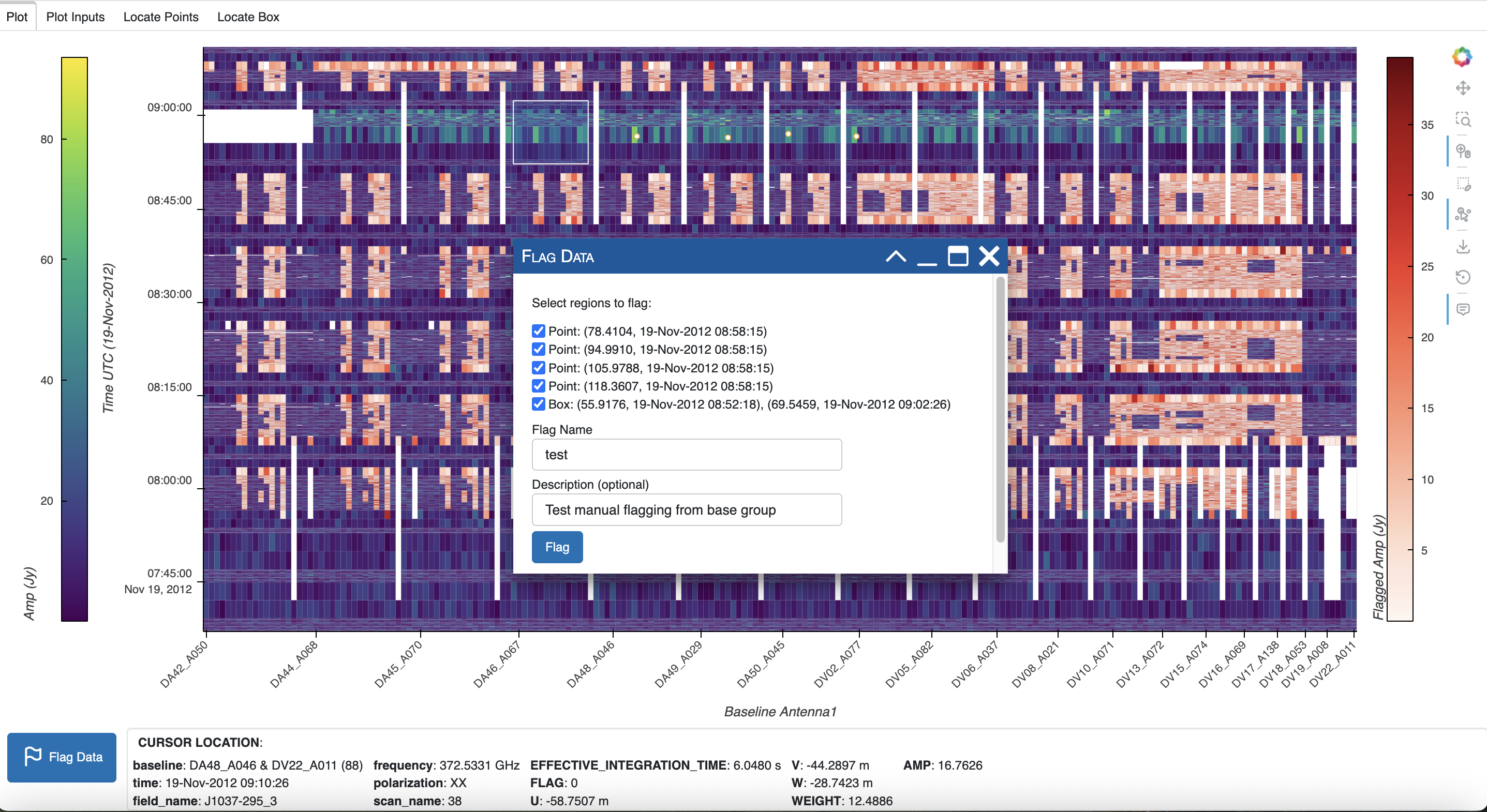
The drawn regions may be selected for flagging by checking the box next to a point or box. The hover tool may be used if needed to identify each point or box on the plot. After one or more regions are selected, input a Flag Name where indicated. This flag name is required and will be used to name a new data variable with the new flags, by prepending FLAG_ with the uppercase Flag Name; for example, if the name test is entered, the new flags will be FLAG_TEST.

In addition, a new data group will be created from the data group selected for the plot, with the lowercase Flag Name. In this example, a data group test will be created with the ‘flag’ key set to FLAG_TEST. In addition, the data group ‘date’ key will be updated with the current date and time. If the optional Description is entered, the data group ‘description’ will be set to this input, else left blank.

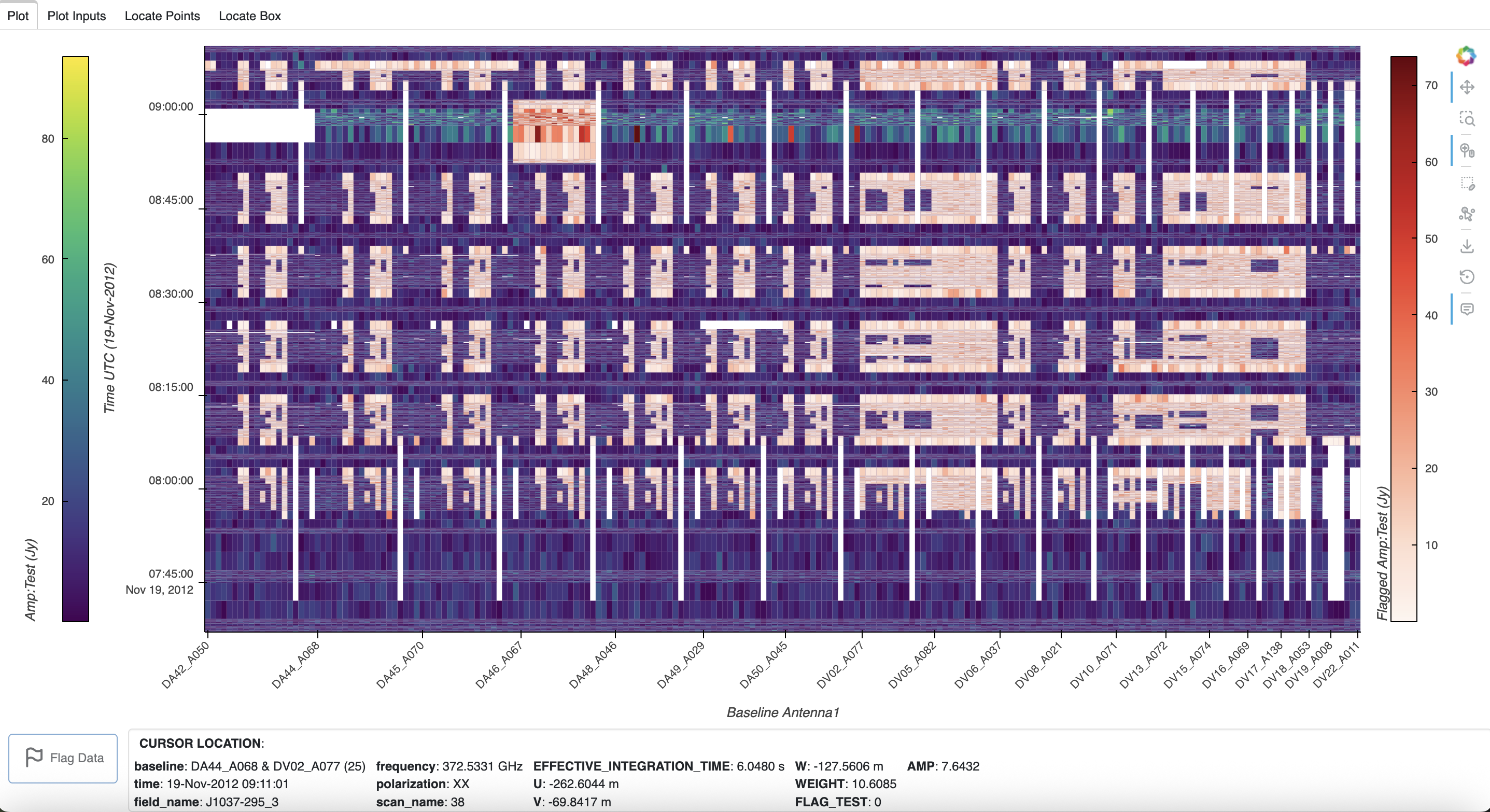
When ready to flag, click the Flag button. If the new flag data variable name exists in the ProcessingSet, an error will pop up and another name may be entered. Otherwise, the current flags are copied to the Flag Name as described above, the flags are set according to the region selection, and the data group is created. The new flags and data group are written to the Zarr file on disk, and a popup notification will indicate the flagging was a success. Then the dialog is closed and the new data group is automatically selected and plotted, as indicated in the data_group listed in the Plot Inputs tab. Note that in the cursor location box, the flag value is listed with the new label FLAG_TEST.

In the Python console, the data groups now include the new test group:

>>> msr.data_groups(True)
base :
    correlated_data = VISIBILITY
    date = 2026-04-29T15:05:27.754696+00:00
    description = Data group derived from the data column 'VISIBILITY' of an MSv2 converted to MSv4
    field_and_source = field_and_source_base_xds
    flag = FLAG
    uvw = UVW
    weight = WEIGHT
test :
    correlated_data = VISIBILITY
    flag = FLAG_TEST
    weight = WEIGHT
    uvw = UVW
    field_and_source = field_and_source_base_xds
    description = Test manual flagging from base group
    date = 2026-05-06T21:27:02.689427+00:00

To go back to the original flags in the base data group, simply clear the selection and select this data group:

>>> msr.clear_selection()
>>> msr.select_ps(data_group_name='base')
>>> msr.plot()
>>> msr.show()

Save Raster Plot

After a plot is created (see Create Raster Plot), it may be saved to a file with save().

>>> msr.save(filename='', fmt='auto', width=900, height=600)

filename (str): name of file to save. Default ‘’ saves the plot as {ms_name}_raster.{ext}). If fmt is not set, the plot will be saved as .png.
fmt (str): format of file to save (‘png’, ‘html’, or ‘gif’). Default ‘auto’ infers the format from filename extension.
width (int): width of exported plot in pixels.
height (int): height of exported plot in pixels.

Multiple plots can be saved in a layout using the subplots parameter of the Create Raster Plot plot() function. Each plot in the layout will have the size (width, height), resulting in a layout plot of size (width * columns, height * rows) pixels. This layout plot is saved to a single file with filename.

However, if iteration plots were created and subplots is a single plot (None or (1, 1)), the iteration plots will be saved individually with a plot index appended to the filename according to the iter_range index range: {filename}_{index}.{ext}. See examples below.

When save() is called, the plot is exported to an HTML file. When fmt is ‘png’, the plot is rendered in memory then a screenshot is captured to create a PNG file. For ‘svg’ export, Bokeh replaces the HTML5 Canvas plot output with a Scalable Vector Graphics (SVG) element that can be edited in image editing programs such as Adobe Illustrator and/or converted to PDF.

Warning

If you have rendered the plot with show(), it is much faster to save the plot with the Bokeh save tool than with save().

Iteration save() examples:

Create plots for the first four frequencies, and save them in a 2x2 layout:

>>> msr.plot(iter_axis='frequency', iter_range=(0, 3), subplots=(2, 2))
>>> msr.save(filename='iter_freq_layout.png')

Create plots for a range of frequencies, and save them individually with an index (in this example: iter_freq_10.png, iter_freq_11.png, iter_freq_12.png, iter_freq_13.png):
```
>>> msr.plot(iter_axis='frequency', iter_range=(10, 13))
>>> msr.save(filename='iter_freq.png')
```
Create plots for all polarizations, and save them individually with an index (in this case, iter_pol_0.png, iter_pol_1.png, etc. depending on the number of polarizations):
```
>>> msr.plot(iter_axis='polarization', iter_range=(0, -1))
>>> msr.save(filename='iter_pol.png')
```

Use Interactive GUI

As mentioned in Construct MsRaster Object, set show_gui to True to launch the interactive GUI. In this case, the ms path can be supplied but is not required.

>>> msr = MsRaster(ms=None, log_level='info', show_gui=True)

The GUI will immediately launch in a browser tab. If ms is set, a plot with default parameters is created and shown in the GUI. As with show(), the plot is shown in the first tab (Plot), the inputs for the plot are shown in the second tab (Plot Inputs), and location information for points selected with plot tools are shown in the remaining two tabs (Locate Selected Points and Locate Selected Box; see Locate Plot Data). By default, the pan, wheel zoom, and hover tools are activated:

Plot Settings:

When using the interactive GUI, settings for the plot may be changed in the Plot Settings tab. This allows the user to set all of the parameters in the MsRaster functions set_style_params, select_ps, select_ms, and plot, described above:

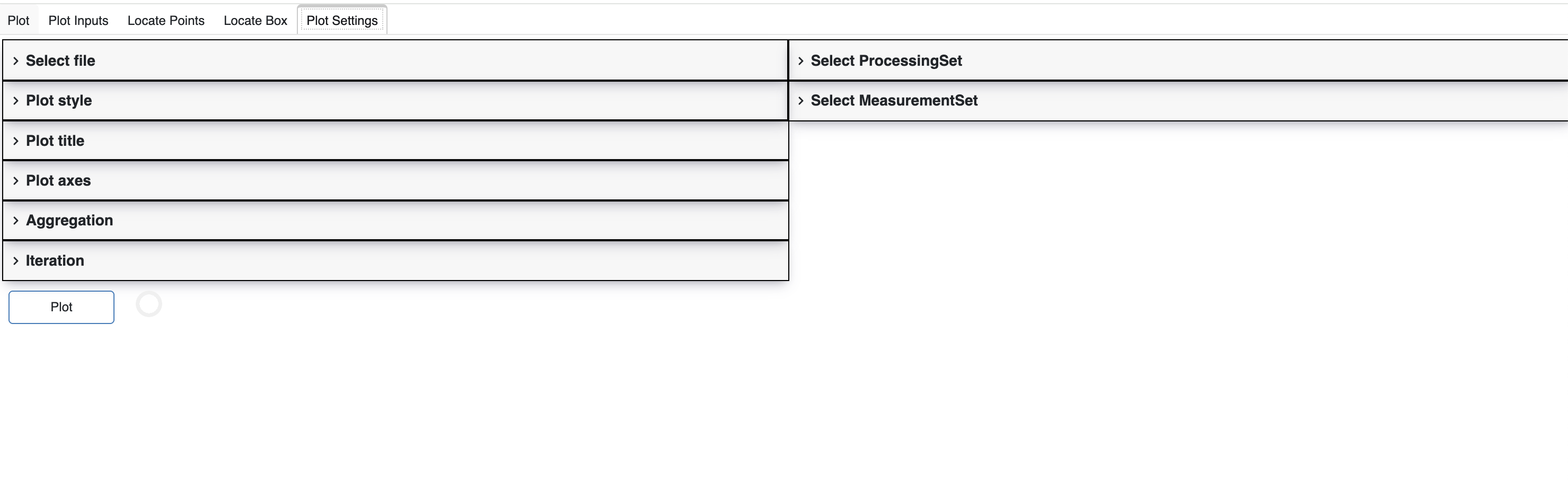
In this accordion-style panel, each section may be expanded to access its settings. The Plot button below the panel will change from outline to solid when the settings change. Click Plot to create the plot. The spinner to the right of the button will rotate until the plot is complete and shown in the Plot tab, with the updated plot inputs in the Plot Inputs tab.

Construct MsRaster Object parameters:
- Select file: ms
Style Raster Plots parameters:
- Plot style: unflagged_cmap, flagged_cmap, show_colorbar, show_flagged_colorbar
Select Raster Data parameters:
- Data Selection:
  - Select ProcessingSetXdt: query, summary column names
  - Select MeasurementSetXdt: data group, dimensions, antenna1 and antenna2
Create Raster Plot parameters:
- Plot axes: x_axis, y_axis, vis_axis
- Aggregation: aggregator, agg_axis
- Iteration: iter_axis, iter_range, subplots
- Plot title: title

Note

Currently, the only way to create multiple plots in a layout is iteration. Iterated plots in a layout will be shown in a new browser tab.